Stability, capability and sigma level of process quality

Stability, capability and sigma level of process quality

Process stability refers to the predictability of the process to remain within control limits (process voice). If the process distribution remains consistent over time, i.e. outputs fall within control limits, then the process is said to be stable or in control. If the outputs are arranged outside the control limits, the process is unstable or out of control.

Process capability is a measure of the ability of the process to meet customer specifications (customer’s voice). The measure tells how good each individual output is. Ppm – part per million is a method for measuring process capability. Ability analysis uses measures such as Cp, Cpk, Pp, Ppk to determine process capability.

The distribution of the mean values of a variable affecting the output quality, specification and control limits are shown in figure 1.

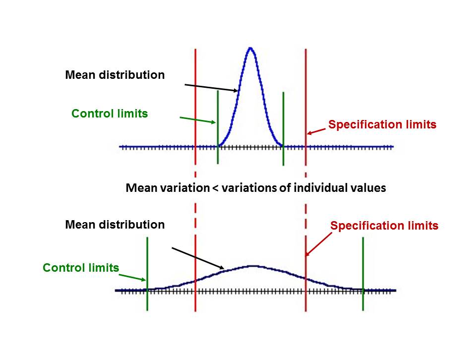
Figure 1 Distribution of mean values, specification and control limits

Process or control boundaries:

• Statistical
• Process boundaries are applied to individual objects
• Control limits are used with mean values
• Limits = μ ± 3σ
• Identify common (common causes) & unusual (special causes)

Specification limits:

• Planned by a buyer or specialist
• Limits = setpoint ± tolerance
• Determine acceptance & non-acceptance

The Gaussian curves for a stable and unstable process are shown in figure 2[1].

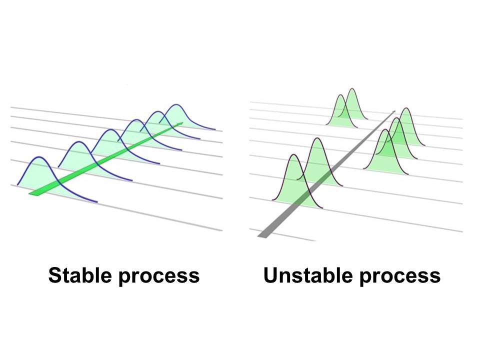
Figure 2 Stable (in control) and unstable process (out of control)

The process could be stable, in terms of meeting customer specifications, but at the same time not capable. This means that the process is stable but stable in producing poor results. In such a scenario, the process in statistical control means nothing in terms of deciding how good or bad the process is. Simply put, stability and ability should be hand-in-hand in terms of interpretation, but at all times the process must be stable before it is capable.

A capable process can be at different levels of ability measured by the level of process quality. Thus, in the 1970s, the quality level was 3 sigma, which meant that 67,000 defects per million opportunities for error occurred. This was unacceptable in terms of profit and competition, so in the late 1980s, Motorola launched the Six Sigma project (Mikel Harry, Ph.D. and Richard Schroeder, Six Sigma: The Breakthrough Management Strategy). Six Sigma quality levels mean 3.4 defects per million error opportunities.

Process stability

The main tool used to evaluate process stability is the control chart. A team leader working to improve process stability and capability must bring together an appropriate team of process owners to work with. With appropriate training, people who work in the process can often collect and interpret control chart data. The assembly of people should be guided and selected by people who have knowledge of the process, who have received training, have the time and appropriate skills to work with control charts.

Control chart

The control chart is similar to the process flow chart. It is also a line graph showing variation over time. Its horizontal axis is the most common time or sequence of measurements. The control map carries much more information, primarily because of the control limits that are calculated on the basis of data – that is the voice of the process.

Control charts help detect the problem signals in the process before a problem occurs. The points on the control chart give an image that can be analyzed to observe the variation of the process.

The control chart is the core of all SPC activities. Only the graphical representation of the measurement values can already be a good estimate of the behavior of the process, and thus the performance of the process quality. Only the application of control charts with control boundaries, pertaining to the process, allows a simple assessment of whether the process is “statistically under control”. Formulas that apply to quality calculations can also be applied when process stability has not been previously proven. The process control type, which is most appropriate for the specific process conditions, should be used to monitor the process. The decision on the most appropriate type of control chart depends on the specific application, in any case, it should be based on existing experience. A tree diagram for selecting a control map is shown in figure 3.

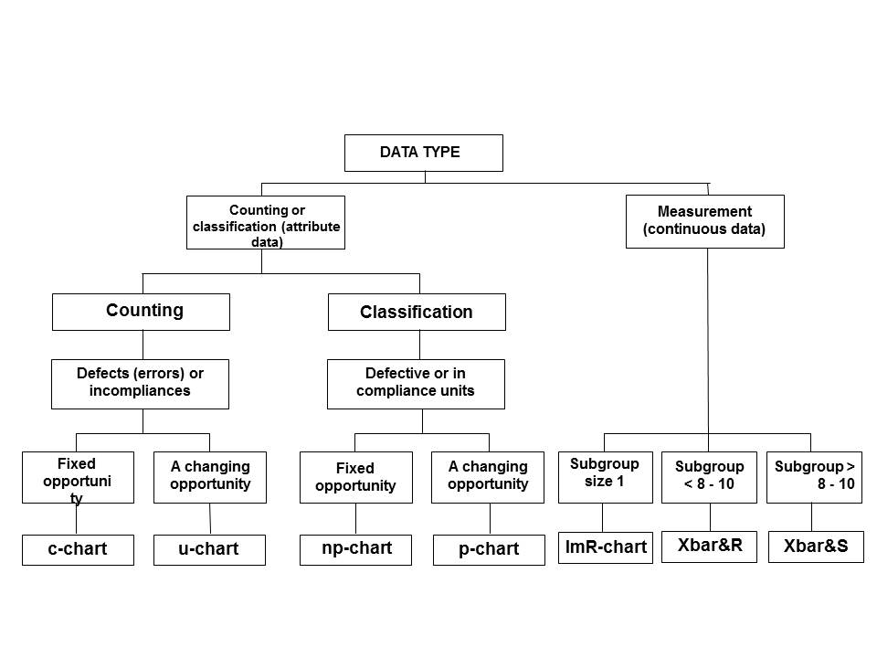
Figure 3 Tree diagram for selecting control charts

Control charts can visualize the behavior of the process with respect to its position and scattering. In addition, features (eg, number of mismatched units, number of errors per unit, original values, mean values, standard deviation, and ranges) are presented to estimate the position and scatter over time and compared with control limits (so-called intervention limits – control).

Process stability calculations

The process and formulas for calculating the process capability for continuous data, normal data, are further provided.

Choice: Cp versus Cpk (or „P“ version)

• C_p and P_p calculations represent a comprehensive comparison of process outputs against desired limits. These computations are constructed separately by comparing the variation of both the upper and lower specification limits. The calculations include the mean, so they are best used when the median is not easily adjusted are based on the full range of variation compared to the specification (it does not compare performance with the mean), so they are best used when:

• the mean can be easily adjusted (such as transactional processes where resources can be easily added so that they have no or minor impact on quality) and
• the mean is monitored (so the process owner knows when adjusting is needed – performing controls is one way of monitoring)

• C_pk and P_pk the computations are constructed separately by comparing the variation of both the upper and lower specification limits. The calculations include the mean, so they are best used when the median is not easily adjusted.

• process improvement efforts may prefer to use Ppk as it is more representative of customer experience over time
• C_pl and C_pu (and P versions) are intermediate steps to determine Cpk

Calculation and interpretation C_pk or P_pk

C_pk is less than C_pu or C_pl (the same for P versions) when the process has an upper and lower specification limit.

• C_pl or P_pl = shows stability when only the lower specification limit exists (for example cooking temperature should not be less than 60 ⁰C to eliminate biohazards)
• C_pu or P_pu = shows stability when there is only the upper specification limit (for example delivery time cannot exceed 24 hours)
• Calculate both values and report a smaller number
• The typical planned score for a capability mark is greater than 1.33 (or 1.67 if security-related)
• Give the highest priority to parameters if the ability is less than 1.00 (need to center the process around specifications, reduce variation, or both)
  • If the process/product is good and there are no problems for the customer, it should be seen whether the defined tolerances can be changed – what is the need for a formal specification if the other “de facto” specification is used for a long time?
  • It may be necessary to perform 100% inspection, measurement and sorting until the process is improved.

The qualification of ability characteristics by value is done according to the following algorithm. If the coefficients C_p and C_pk  (figure 4):

• at least one less than 1 is said to be incapable of the process.
• both greater than or equal to 1 and less than 1.33, the process is said to be conditionally capable,
• both greater than or equal to 1.33 and less than 1.67, we say the process is capable,
• both greater than or equal to 1.67 for the process is said to be excellent capable,

Process capabilities ranging from Cpk = 1 to Cpk = 2 are shown in Figure 4 and give an example of a car entering a garage. If the width of the entrance to the garage is the same as the width of the car, it is clear that there will be a left or right locking in any unforeseen impact (shifting by + – 1.5 sigma). If the width of the entrance to the garage increases to 1.33 the width of the car, the chance of damage to the car at the entrance to the garage is less. Finally, if the width of the entrance to the garage is 2 times the width of the car, in this case, the novice driver will be able to import the car without hooking the left or right edge of the entrance – up to 6 sigma quality level. The same goes for the process. If the small standard deviation

The Gaussian curve will be within the specification limits. The smaller the standard deviation, the more capable the process is.

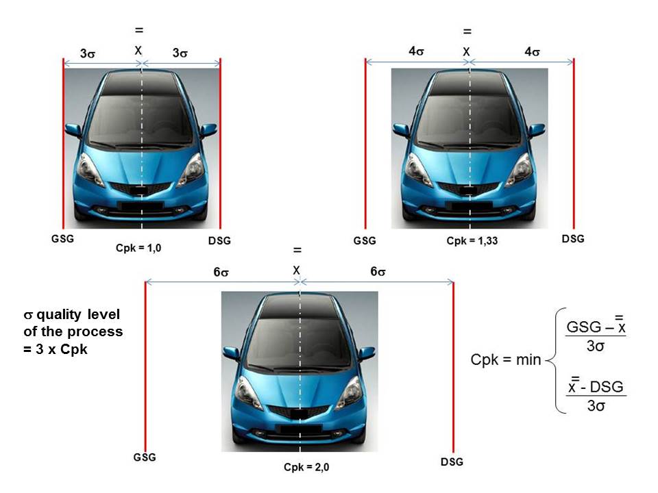
Figure 4 Demonstration of process capability in the range from Cpk = 1 to Cpk = 2 in the example of the width of the entrance to the garage where the car is parked

The sigma quality level of the process

Processes implemented in any industry require that they are simplified first by applying the Lean concept and then reducing the variation in output-critical characteristics using the Six Sigma concept. The implementation of the Lean concept should make it possible to eliminate non-value-added activities and then reduce or eliminate some of the 8 major wastefulness that occurs in the process.

There are two causes for variations to occur:

General causes:

• Random variation (common)
• No template – a pattern
• Inherent in the process
• Adjusting the process increases its variation

Special causes:

• Not a random variation (unusual)
• Can show a pattern – template
• Assignable, they can be explained, they can be controlled
• Adjusting the process reduces its variation

As activities that do not add value and reduce or eliminate wastage are removed from the process, it is necessary in the next stage to bring the process to a stable state and then to begin its “healing” in order to reduce variations and achieve more ability. The ultimate goal should be to reach Six Sigma quality levels, which means 3.4 errors per million error opportunities.

The process sigma quality level, expressed through defects per million error opportunities, ranged from 66,807 in the 1970s to 3.4 errors in the late 1980s when Motorola launched the Six Sigma Quality Level project.

It should be noted here that due to the effect of external factors, the Gaussian curve can be shifted by + – 1.5 sigma (for example, snow on the landing runway or strong wind which can cause the plane to slide to one side or the other and not be safe landing) relative to the target value (Figure 5). In order to prevent the process from becoming incompetent under these conditions, ie to go beyond the specification limits, it is necessary that the process capability is to remain within the specification limits even at such displacement (so that the aircraft does not slip off the runway)).

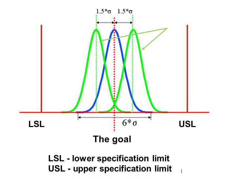
Figure 5 Process shift in the sequence of external factors

Six Sigma is a method that minimizes process variations and provides high new quality on exit. The method refers to the standard deviation of the Gaussian normal distribution. 3 Sigma has 66,807 defects per million options (DPMO). This means 66,807 error opportunities, not faulty products or errors per million error opportunities. The product may have more than one defect.

Quality development over the centuries has ranged from the lowest s level, over 3 sigma quality levels in the 1970s to 6 sigma quality in the last more than 20 years (Figure 6).

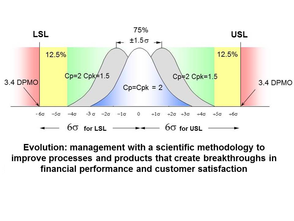
Slika 6 Evolucija sigma nivoa kvaliteta

 

Table 1 shows the Sigma quality level

	No shift 1,5 sigma		With shift 1,5 sigma
Sigma quality level	Defects per a million opportunities for error – DPMO	Yield	Defects per a million opportunities for error – DPMO	Yield
1	317.310	68,2690000%	697.612	30.23880%
2	45.500	95,4500000%	308.770	69,12300%
3	2.699	99,7301000%	66.810	93,31900%
4	63	99,9937000%	6.209	99,37910%
5	0,574	99,9999426%	232	99,97680%
6	0,002	99,9999998%	3,4	99,99966%

 

As shown in Figure 2, the values are given in the case of shifting the Gaussian curve for +- 1,5 sigma.

One realistic example of a control chart, with data and a Histogram, for a process whose ability Cpk = 2.32089 (process quality greater than 6) is shown in Figure 5. From the figure, it can be seen that the Gaussian curve is slightly shifted to the right and Cpk is larger of Cpk and is 2.7832999). The process sigma quality level can be calculated by multiplying the Cpk process capability by 3 sigma which equals sigma = 6.96267. For this realistic process and one characteristic quality feature, it is seen that this is even higher than the Six Sigma process quality level. This can also be seen from a visual representation of a Gaussian curve that is shifted significantly within the specification limits (Figure 7).

Figure 7 Real-life example of a control chart with data and a Histogram

Assumptions for interpreting control charts

„Special Causes Test “assumes that there is a normal distribution of data.

• The control limits are – standard deviations from the mean, and calculating the standard deviation assumes the existence of a normal distribution of data

• If the distribution of the drawn points is not normal, control limits cannot be used to detect uncontrolled conditions
• To fix the problem, use the central limit theorem to determine which sample size of the subgroup will allow the average values of the normally distributed data to be plotted.

All tests for special causes also assume that they are independent observations.

• Independence means that the value of any data point is not affected by the value of another data point
• If the data is not independent, the data values will not be random
• This means that the rules for determining the specific cause of the variation will not be enforceable (because they are based on the rules of statistical randomness)

Many of the tests are linked to “zones” that indicate standard deviations from the mean. Zone C is  +- 1 sigma – standard deviation; zone B is between  +- 1 sigma and  +- 2 sigma standard deviation and zone A is between  +- 2 sigma and +- 3 sigma – standard deviation. Someone marks the zones in the second row, that is, zone A is +- 1 sigma – standard deviation; zone B is between +- 1 sigma and  +- 2 sigma – standard deviation and zone C is between +- 2 sigma and +- 3 sigma – standard deviation (Figure 8).

Figure 8 Zones denoting standard deviations s

There are two types of rules as methods for controlling a process when determining whether a measured variable is out of control (unpredictable versus consistent).

Rules for detecting “out of control” or non-random conditions were first discovered by Walter A. Shewhart in the 1920s. There are two types of rules and:

• Nelson rules
• The Western Electric rules

Nelson’s rules are a method of process control in determining whether a measured variable is out of control (unpredictable versus consistent). Nelson’s Rules were first published in November 1984 in the Journal of Quality Technology in an article by Lloyd S Nelson [2].

Western Electric Rules are decision rules in the statistical control of processes for detecting out of control or non-random causes on control charts. The points of observation with respect to the control limits of the control map (usually to ± 3 standard deviations) and the center lines indicate whether the process in question needs to be investigated for assignable causes. The rules of Western Electric were codified by the specially appointed commission of the production division of the Western Electric Company and appeared in the first edition of the 1956 manual, which became the standard text of the field. Their purpose was to ensure that line workers and engineers interpret control charts in a unique way[3].

Interested experts can get acquainted with the rules in the above references.

The physical and digital process model (twin model)

The physical model of the process, discussed in the previous points, is a realistic model of the process. This process model can be monitored using classical approaches (the DMAIC process in the Six Sigma concept) and controlled by control charts that show whether the process is stable and capable of the process, ie what the quality level of process quality is. The disadvantage of this model is that it monitors the individual characteristics critical to output quality without taking into account the interplay.

To solve this problem, when a huge amount of data (BIG DATA) can be acquired through the sensor, a digital model of the process has come up. The Digital Twin Transformation Model aims to address the benefits and impacts of critical process features in manufacturing, including implementation strategies. The concept of a digital process model (Twin model) enables manufacturing industries to grasp the impact of output-critical features, improve productivity and operational efficiency while optimizing the maintenance process, required resources, time and cost.

Advances in information technology have made it possible to develop BIG DATA ANALYSIS and thus obtain the Digital Twin production process. This leads to smart manufacturing becoming the focus of global manufacturing transformation and upgrading (Industry 4.0). By applying this approach, analyzing a large amount of data, one obtains knowledge from that data, which allows one to initiate improvement and attainment of a high  level of process quality. The analysis of large quantities of production data is useful for all aspects of production. Figure 9 shows real and digital world models.

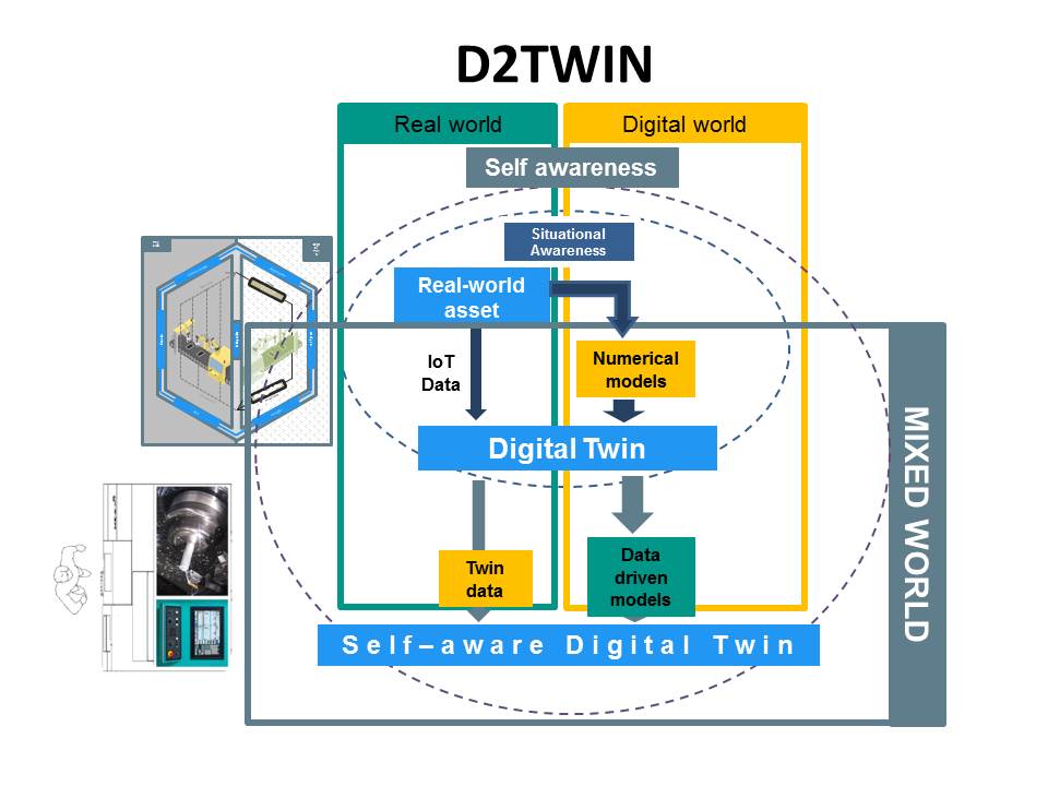
Figure 9 Real and digital world

The Internet of Things (IoT) creates a tremendous amount of data that is currently retained in vertical silos. However, true IoT is dependent on the availability and acquisition of large amounts of data from multiple systems, organizations, and verticals that are introducing a new generation of Internet solutions.

In production, BIG DATA includes a large volume of structured, semi-structured and unstructured data generated from the product life cycle. The increasing digitization of production is opening up opportunities for smart manufacturing. Production data is collected in real-time and automatically sent to the appropriate server, which does not have to be located at the location where the production takes place. Through the analysis of this data based on cloud computing, one can look at the problems that occur in manufacturing from bottlenecks in the manufacturing process, through problems with tool wear, increased temperature, machine maintenance and the like. Based on such analyzes, experts can propose solutions for how to improve the manufacturing process, extend the time of using expensive tools, reduce or eliminate unnecessary maintenance prescribed by the equipment manufacturer and the like. In this way, it is possible to achieve production that is more and leaner and without variations. All valuable information from big production data is feedback on product design, production, planning of required materials (maintenance, repair, and overhaul), etc. It is a way to achieve smart manufacturing.

A 3D representation of the cluster, after analyzing a large amount of data on one example of mass production of engine block screws, is shown in Figure 10. Each color in Figure 10 represents a cluster of some of the process quality critical features.

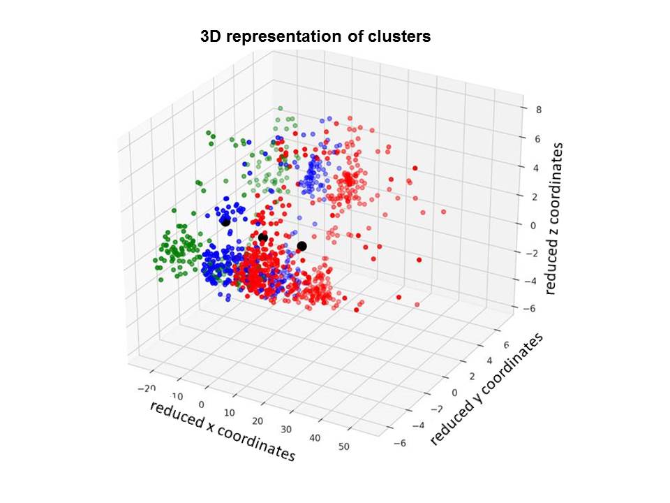
Figure 10 3D representation of the cluster

Physical fashions provide knowledge of what action can be taken. On the other hand, the knowledge gained from the digital model explains why something happened in the process. In the example shown in Figure 11, the problem in the process of manufacturing the engine block bolts was due to tool wear. Available knowledge for action can trigger an action related to a change in some of the characteristics that are critical to the quality of the output, but that action, due to the influence of other characteristics, will not lead to improvements, but to a deterioration of the process. On the other hand, the knowledge extracted from the analysis of a large amount of data indicates exactly WHY something happened. On this basis, it is possible to take appropriate action, in this case, to replace the worn tool.

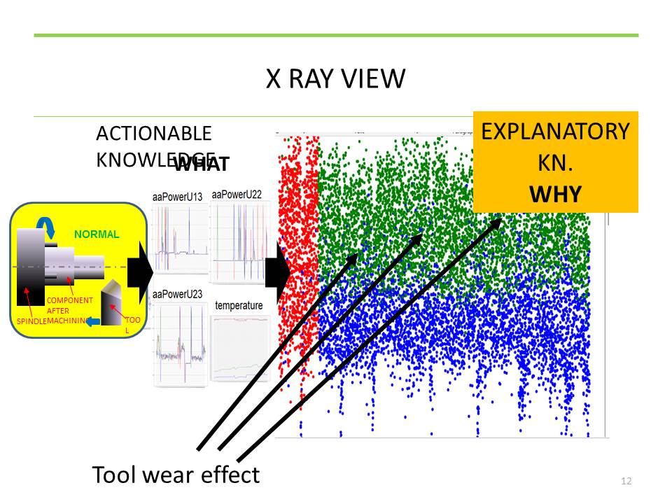
Figure 11 Available knowledge for action and knowledge that explains why something happened

Conclusion

Digital twins create digital models of physical objects in a digital way to simulate their behavior. Digital models can understand the state of physical models (why something happened) through data collected from sensors. In the example shown in Figures 9 and 10, 4 sensors were used to record the data, which continuously and directly acquired the data from the process of manufacturing the screws for the engine block. In this way, the digital model can achieve optimization of the entire production process, as opposed to the physical model that can achieve optimization of certain characteristics critical to the production process.

Note: This work has been published by the author in Serbian on this blog on 01/22/2019. years. Google Analytics has shown that this work is also accompanied by visitors who are not from the Serbian speaking market. The author, therefore, decided to present this work in English.

 

At Nis, 14.11.2019.                                               Prof.dr Vojislav Stoiljković

[1] https://www.winspc.com/what-is-the-relationship-between-process-stability-and-process-capability/

[2] https://en.wikipedia.org/wiki/Nelson_rules

[3] https://en.wikipedia.org/wiki/Western_Electric_rules